NPBayesHMM

Welcome to the NPBayesHMM toolbox

This is a Matlab toolbox for performing inference on collections of sequential data. For example, you can analyze several motion capture sensor streams at once, or find common activities in a video corpus.

The basic model we employ is the Beta Process Hidden Markov Model (BP-HMM). Briefly, this model assumes that each sequence is generated by a "hidden state sequence" (technically, an HMM), which indicates which of a global set of possible behaviors (think mocap exercises) is active at each time. Once we know the active behavior at time t, we generate the observed data at that step from its behavior's emission distribution. This model assumes exactly one behavior is active at each step.

Unlike the usual HMM approach, our BP-HMM is nonparametric. This means that it does not require specifying in advance the exact number of behaviors used. Instead, our inference explores possible sets of behaviors and finds an appropriate fit in a data-driven way. This toolbox exists because these kinds of inference algorithms are quite complicated. We've developed state-of-the-art methods to fit these models to real data, successfully analyzing hundreds of sequences at once.

For academic descriptions of our models and inference algorithms, see our Academic Citations

Installation

For complete details, check out the plain-text Quick Start Guide

1. Install required libraries
   • Eigen C++ Matrix Library
   • Tom Minka's Lightspeed for Matlab
2. Compile MEX functions for fast HMM dynamic programming
   • See HOME/code/CompileMEX.sh for details
3. Specify where you want saved results.
   • Create file HOME/code/SimulationResults.path
   • Add one line of text that's a valid path on local system.

Dive in!

The best way to understand the toolbox is to check out the demos in HOME/code/demo/. Here, we'll walk through the simplest, EasyDemo.m.

First, open Matlab and set up the working directory. Then just run the demo!

>> cd <path/to/NPBayesHMM/HOME>/code/

>> configNPBayesToolbox(); % adds paths appropriately

>> EasyDemo();

First, a collection of 5 data sequences are generated. Here are two of them. They are each 500 timesteps long, and at each timestep we observe a 2-dimensional vector (black and red lines).

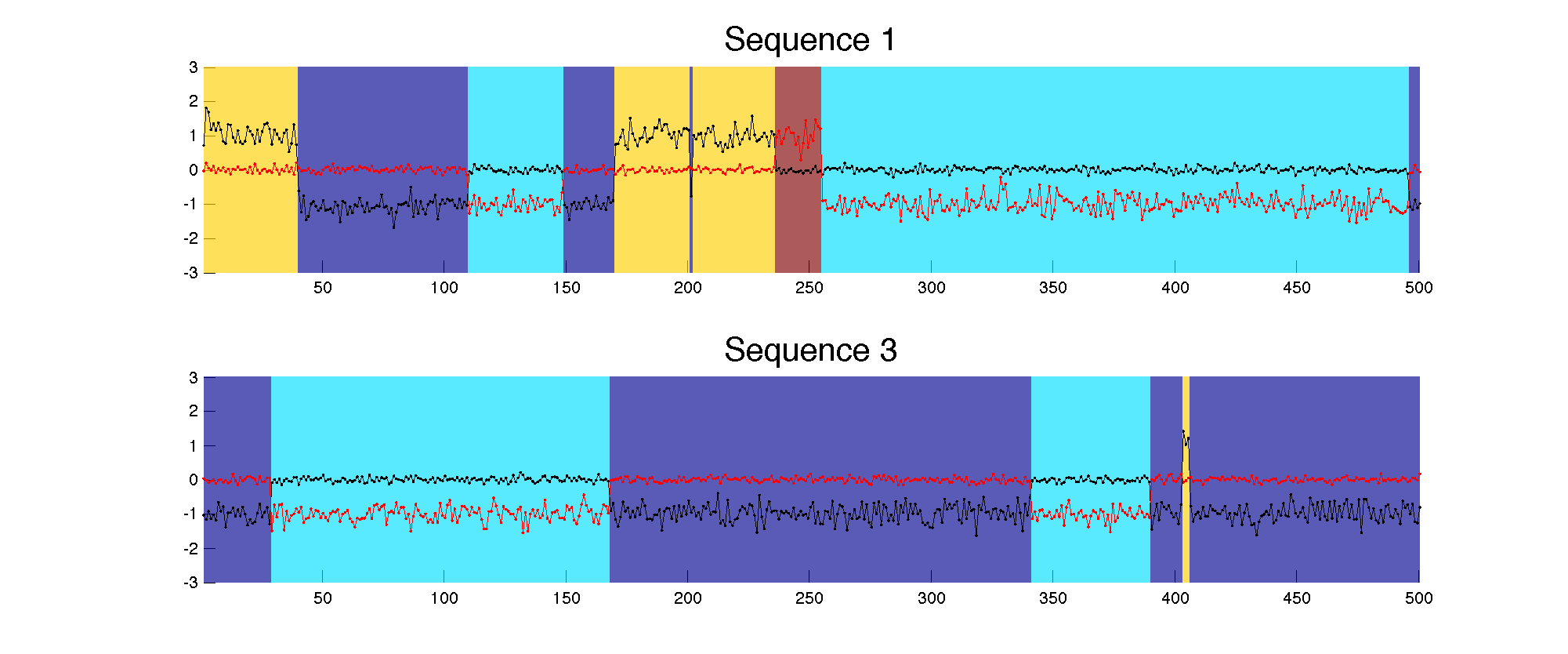
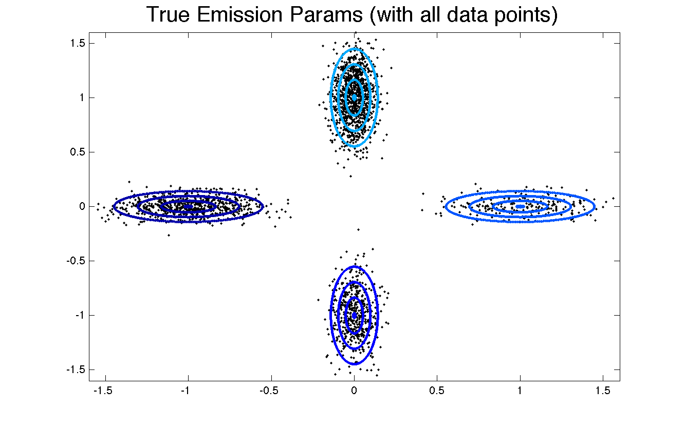
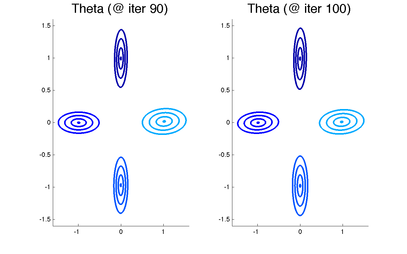
This data was generated by 4 hidden "behaviors" (also called features). The background color specifies which behavior is active at each timepoint. Each behavior specifies a 2D Gaussian distribution, which serve as the emission parameters when the HMM is actively in that state. In this toy example, these 4 behaviors have well-separated parameters, as seen in this contour plot.

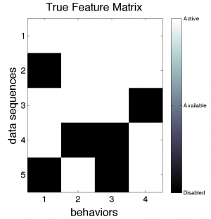
We can build a binary matrix that indicates which sequences use which behaviors. We call this matrix F, for "feature matrix".

Running MCMC

After generating this data, we apply our posterior inference algorithm to learn the emission parameters theta and feature matrix F. This demo performs 100 iterations of MCMC.

The amazing thing out our nonparametric approach is that we do not need to specify the number of features... we can start the inference with just one feature and the algorithm will explore until it finds the best possible set of features. You can see this in the stdout feed produced by the inference.

Initial Config: 
         0/100 after      0 sec | logPr -5.21e+03 | nFeats    1 
Running MCMC Sampler 1 : 1 ... 
         1/100 after      0 sec | logPr -3.97e+03 | nFeats    3 
        10/100 after      1 sec | logPr  2.71e+03 | nFeats    5 
        20/100 after      1 sec | logPr  2.72e+03 | nFeats    4 
        30/100 after      1 sec | logPr  2.72e+03 | nFeats    4 
        40/100 after      1 sec | logPr  2.72e+03 | nFeats    4 
        50/100 after      2 sec | logPr  2.72e+03 | nFeats    4 
        60/100 after      2 sec | logPr  2.72e+03 | nFeats    4 
        70/100 after      2 sec | logPr  2.72e+03 | nFeats    4 
        80/100 after      3 sec | logPr  2.72e+03 | nFeats    4 
        90/100 after      3 sec | logPr  2.72e+03 | nFeats    4 
       100/100 after      3 sec | logPr  2.72e+03 | nFeats    4 

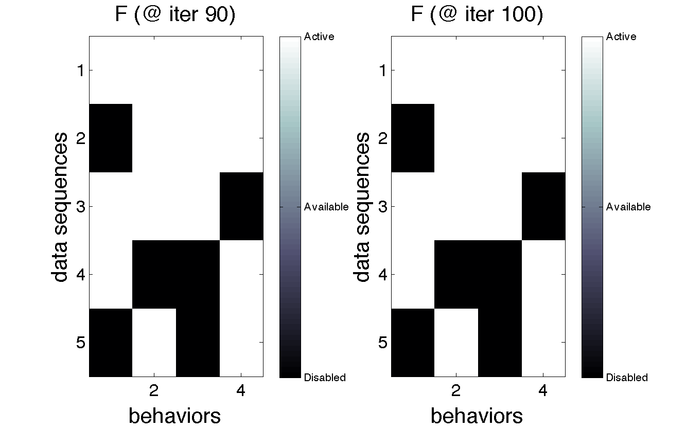
Here's a look at the recovered Feature matrix:

The recovered emission parameters theta:

Finally, the recovered state sequence for the two sequences we plotted earlier

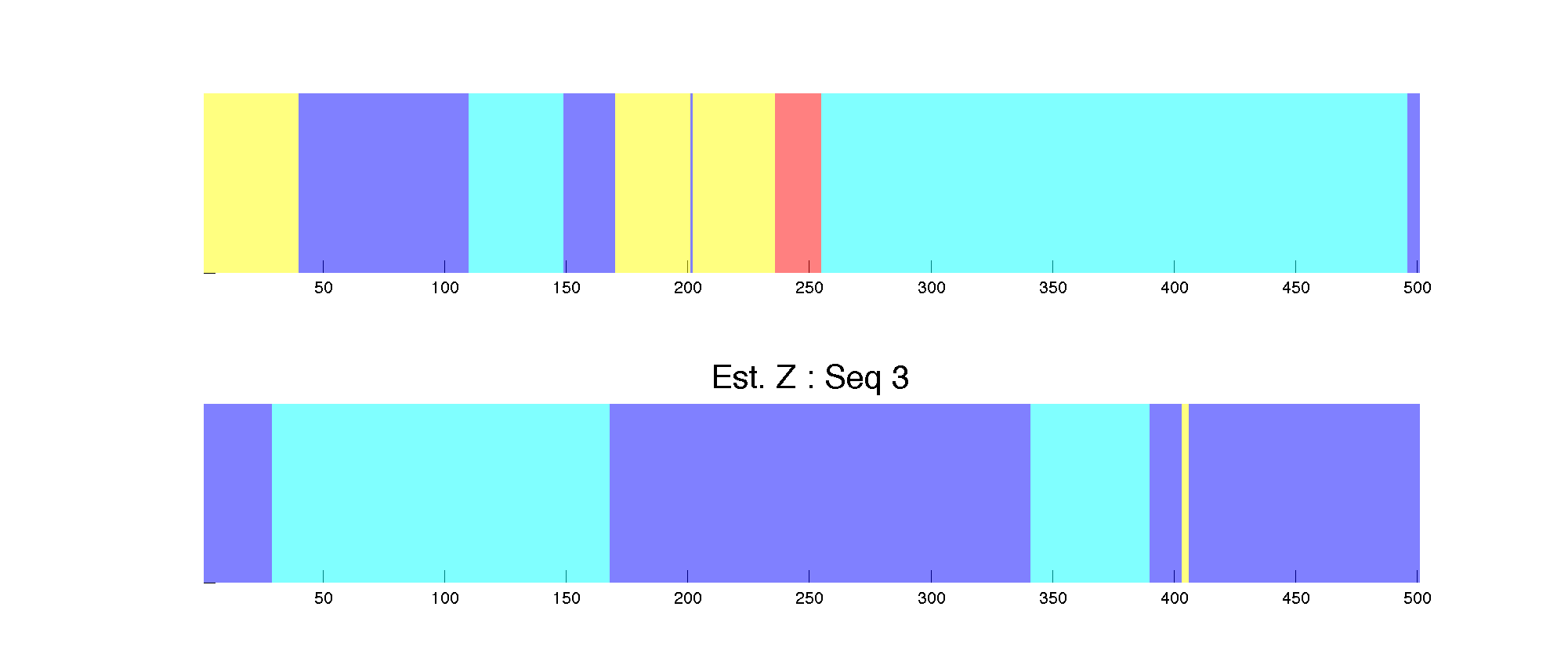
That's it! Hopefully this demo convinced you that (1) our inference works, and (2) the NPBayesHMM toolbox can be a productive tool for analyzing sequential data.

More information

Contact Mike Hughes via email: mike <AT> michaelchughes.com

Related Projects

Check out Matthew Johnson's HDP-HSMM project: https://github.com/mattjj/pyhsmm

Also, see Emily Fox's original BP-AR-HMM toolbox: http://www.stat.washington.edu/~ebfox/software.html